Vehicles with conventional steering mechanisms like Ackermann steering and differential-drive serve distinct purposes. With wheels engineered to maintain constant contact with a driving surface, these vehicles navigate reliably between destinations, albeit with a restricted range of directional movement. A swerve-drive provides an approach with significantly more freedom.

For dozens of navigation use cases, these conventional steering methods are sufficient. But a swerve-drive is exceptionally helpful in tight spaces like the one Mike Meyers faced in Austin Powers: International Man of Mystery, and in general, where holonomic capabilities would help. 

Swerve-drive is an omnidirectional (‘all directions’) drive-train in which all wheels are independently steered and driven. This  allows vehicles to spin on a spot, drive sideways (strafing), diagonally, or at other angles that aren’t possible with Ackermann steering or differential drive.

This post explores the intricacies of swerve-drives, explained within the context of a robot we are developing at Fresh. Specifically, we will cover:  

• The benefits of swerve-drives and omnidirectional steering
• The challenges of implementing a swerve system
• A dive into the math involved in setting up a swerve-drive, 
• Dockerized simulation and source code for swerve-drive kinematics and odometry
  

For anyone working in transportation, construction, or dozens of other fields that benefit from automation and robotics, the value of implementing such a system speaks for itself. With swerve-drive, vehicles and machines can move in entirely new ways, as depicted in the video below.

Benefits of Swerve: Omni-directional steering, reliability on ‘non-ideal’ surfaces, and streamlined maintenance

Let’s quickly cover the benefits of swerve:

• Agility: Drive direction is independent from chassis orientation i.e the vehicle doesn’t need to face the direction it intends to travel in, thus these swerve-drive vehicles have a larger range of motion.

• Traction: The “drive force” can be vectored in any direction. High traction wheels can be used, unlike mecanum wheels which suffer from power loss. 

• Outdoor use: Swerve-drives are suitable for outdoor use; mecanum wheels need level ground.

• Flexibility: Ability to operate in different drive modes switchable through software. Serves as a single platform to test control and navigation algorithms for the different drive modes.
• Serviceability: The system is modular; each swerve module can be swapped out if needed.

Swerve-Drive Drawbacks: Complex, expensive, and highly-technical

Swerve is not mainstream as of yet, and there are inherent costs. In the interest of transparency, let’s discuss the downsides:

• Mechanical complexity: Swerve-drive is difficult to design.

• Software complexity: Swerve-drives are challenging to implement. It requires enforcing physical constraints in controls software to ensure all 8 motors work in sync so as to not pull the robot apart.
• Equipment complexity: Swerve requires 8 motors (4 drive + 4 steering) and eight corresponding motor encoders. There is technical debt and the necessity of a higher build budget.

Two clear-cut swerve-drive use cases

Before we transition into a discussion of the math behind building a swerve-drive, let’s discuss use cases. Across a range of industries, swerve makes sense.

Warehouses, construction yards, and other high-traffic areas

To increase storage in warehouse, dense layouts make sense. To increase efficiency in crowded work settings, more flexible motion primitives would be beneficial. Swerve-drive provides the advantage of both docking and navigating in tight spaces. With holonomic capabilities, vehicles are no longer confined to traditional traffic lanes, opening up new possibilities for transportation, material delivery, and much more.

Outdoor and indoor settings where mecanum suffers from power loss, lower efficiency and low reliability

Wherever mecanum wheels are being used, swerve-drive is something to consider. Mecanum wheels need level ground to work. Whenever strafing with a mecanum wheel vehicle, a portion of power is lost due to the inherent slippage that occurs by design. Swerve-drive can work outdoors on uneven surfaces and provide more traction while being more reliable.

Guidelines for creating a swerve-drive

Now that we’ve covered the basics of what a swerve-drive is and why it should be of interest to those who work with robots, let’s discuss the How-To. This section will cover the math needed to create a swerve-drive.

Kinematics: Deriving commands for the 8 motors from the Twist message

Assume an arbitrary case where a robot receives a Twist message comprising of:

• Linear component along x axis (Twist.linear.x) – $v_x$
• Linear component along y axis (Twist.linear.y) – $v_y$
• Angular velocity about z axis (Twist.angular.z) – $\omega_z$

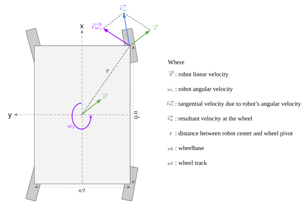
The resultant linear velocity at the wheel is given by the vector sum of the robot’s linear velocity ( $v_x$ & $v_y$ ) and tangential component of the angular velocity ( $\omega_z$ ).
$$ \overrightarrow{v_w} = \overrightarrow{v} + \overrightarrow{r\omega_z} $$
Considering the front right wheel, breaking down the resultant linear velocity in x & y components:
$$ v_{fr_x} = v_x + r_x\omega_z $$ $$ v_{fr_y} = v_y + r_y\omega_z $$
Similarly these equations can be derived for the other wheels ( fr: front_right, fl: front_left, rl: rear_left, rr: rear_right ). Putting all equations in matrix form.
$$ \begin{bmatrix} B \end{bmatrix} = \begin{bmatrix} A \end{bmatrix} \begin{bmatrix} X \end{bmatrix}$$ $$ \begin{bmatrix} v_{fr_x}\\ v_{fr_y}\\ v_{fl_x}\\ v_{fl_y}\\ v_{rl_x}\\ v_{rl_y}\\ v_{rr_x}\\ v_{rr_y} \end{bmatrix} = \begin{bmatrix} 1 & 0 & r_x\\ 0 & 1 & r_y\\ 1 & 0 & -r_x\\ 0 & 1 & r_y\\ 1 & 0 & -r_x \\ 0 & 1 & -r_y\\ 1 & 0 & r_x\\ 0 & 1 & -r_y \end{bmatrix} \begin{bmatrix} v_x\\ v_y\\ \omega_z \end{bmatrix} $$
Where $r_x = wb/2$ and $r_y = wt/2$.

Determine the steering angle ( $\Phi_w$ ) and angular speed ( $\omega_w$ ) for all wheels. Taking an example for the front right wheel.
$$ Steering \; Angle \; \Phi_{fr} \; (rad) = \tan^{-1}(\frac{v_{fr_y}}{v_{fr_x}})$$ $$ Wheel \; Angular \; Velocity \; \omega_{fr} \; (rad/s) = \frac{\sqrt{v_{fr_x}^{2} + v_{fr_y}^{2}}}{radius_{wheel}}$$

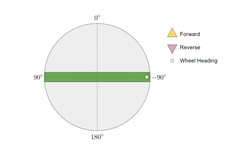
Optimal Wheel Steering

Consider a situation where the wheel heading is -90 degrees as shown in below figure.

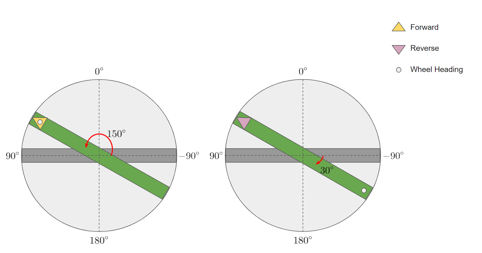
Next, it is desired to head towards 60 degrees. There’s two ways it can be done. In the figure below on the left, the wheel rotates from -90 degrees to 60 degrees heading (turning a total of 150 degrees) and drives forward. It is optimal to instead rotate to -120 degrees heading (turning only 30 degrees) and drive in reverse. 

Wheel Odometry

It is important for robots to know their position. Robots estimate their position using localization algorithms which utilize measurements taken from various sensors as input. One such measurement is wheel odometry which is computed from the wheel encoders. Wheel odometry is one of the measurements which are internal to the robot. i.e., It does not directly depend on the environment. 

Odometry is the relative change in position over time. It is estimated by integrating velocity measurements over time. However, one of its limitations is that the error keeps accumulating causing the position estimate to drift over time.

The procedure to compute odometry can be broken down into two parts:

• Compute twist from joint_states
• Update pose over time using the computed twist

Computing Twist from Joint States

Assuming the robot hardware is setup to publish the joint states or a joint_state_broadcaster for the sim. A ROS JointState message reports the position, velocity and effort of that joint.

We obtain the angular velocity ( $\omega_w$ ) from each wheel joint state and steering angle ( $\Phi$ ) from the steering joint state. Substituting those values in the above equations in the kinematics section that were used to determine the wheel angular velocity & steering angle and solving for wheel linear velocity components, it yields the following equations. Taking front right wheel as an example:
$$ v_{fr_x} = \omega_{fr} * radius_{wheel} * cos(\Phi_{fr}) $$ $$ v_{fr_y} = \omega_{fr} * radius_{wheel} * sin(\Phi_{fr}) $$
Similarly compute the x & y components for all wheels.

Note: If using the optimal wheel steering logic, then it needs to be inverted for computing odometry. Therefore, if a particular wheel’s velocity is negative, then multiply it by -1 and add $\pi$ radians to the steering angle for that wheel.

Solving the above equations for all wheels yields the ‘B’ matrix which was defined in the kinematics section. The ‘A’ matrix is known since it depends on the geometry of the robot. Therefore the only unknown is the ‘X’ matrix which consists of the components of a planar twist.
$$ \begin{bmatrix} B \end{bmatrix} = \begin{bmatrix} A \end{bmatrix} \begin{bmatrix} X \end{bmatrix}$$ $$ \begin{bmatrix} v_{fr_x}\\ v_{fr_y}\\ v_{fl_x}\\ v_{fl_y}\\ v_{rl_x}\\ v_{rl_y}\\ v_{rr_x}\\ v_{rr_y} \end{bmatrix} = \begin{bmatrix} 1 & 0 & r_x\\ 0 & 1 & r_y\\ 1 & 0 & -r_x\\ 0 & 1 & r_y\\ 1 & 0 & -r_x \\ 0 & 1 & -r_y\\ 1 & 0 & r_x\\ 0 & 1 & -r_y \end{bmatrix} \begin{bmatrix} v_x\\ v_y\\ \omega_z \end{bmatrix} $$

Solving for ‘X’ matrix, we have 8 equations and 3 unknown, therefore it is an over-determined system. It can be solved by the QR decomposition method.

For a system, $ \begin{bmatrix} B \end{bmatrix} = \begin{bmatrix} A \end{bmatrix} \begin{bmatrix} X \end{bmatrix}$

• Factorize matrix ‘A’ such that $ \begin{bmatrix} A \end{bmatrix} = \begin{bmatrix} Q \end{bmatrix} \begin{bmatrix} R \end{bmatrix}$ where ‘Q’ is an orthogonal matrix and ‘R’ is an upper triangular matrix.
• Multiply both sides of the system by the transpose of A matrix $ \begin{bmatrix}A \end{bmatrix}^T$:
  $$\begin{bmatrix}A \end{bmatrix}^T \begin{bmatrix}A \end{bmatrix} \begin{bmatrix}X \end{bmatrix} = \begin{bmatrix}A \end{bmatrix}^T \begin{bmatrix}B \end{bmatrix}$$
• Substitute $ \begin{bmatrix} A \end{bmatrix} = \begin{bmatrix} Q \end{bmatrix} \begin{bmatrix} R \end{bmatrix}$:
  $$\begin{bmatrix}R \end{bmatrix}^T \begin{bmatrix}Q \end{bmatrix}^T \begin{bmatrix}Q \end{bmatrix} \begin{bmatrix}R \end{bmatrix} \begin{bmatrix}X \end{bmatrix}= \begin{bmatrix}R \end{bmatrix}^T \begin{bmatrix}Q \end{bmatrix}^T \begin{bmatrix}B \end{bmatrix}$$
• Simplifying
  $$\begin{bmatrix}R \end{bmatrix} \begin{bmatrix}X \end{bmatrix} = \begin{bmatrix}Q \end{bmatrix}^T \begin{bmatrix}B \end{bmatrix}$$

This yields a set of equations which are no longer over-determined and can be solved by any linear equation solver.
QR decomposition solves the overdetermined system by minimizing the sum of squares of residuals in each equation, therefore minimizing the error in estimation of Twist which reduces the drift in odometry. QR decomposition is slightly less efficient than LU factorization but it is numerically stable.

Pose Update

• Initialize the pose components to zeros:
  • $x= 0$
  • $y = 0$
  • $\theta= 0$
• x-coordinate update: $$x= x + [v_x cos(\theta) – v_y sin(\theta)] \Delta t $$
• y-coordinate update: $$y= y + [v_x sin(\theta) + v_y cos(\theta)] \Delta t $$
• heading ( $\theta$ ) update: $$ \theta = \theta + \omega_z \Delta t $$
  where $\Delta t$ is the time interval between joint state updates which is computed from the timestamps in the header of JointState messages.

Swerve-Drive in Simulation

1. Set up a robot URDF with four position-controlled steering joints and four velocity-controlled wheel joints.

2. Swerve control script (swerve_commander.py):
   1. Set up a /cmd_vel subscriber and eight joint controller (4 position + 4 velocity) publishers. 
   2. On receiving each Twist message, compute the wheel velocities and steering angles based on the algorithm above.
   3. Publish computed wheel velocities and steering angles to respective joint controllers.
3. Odometry script (swerve_odometer.py):
   1. Set up a joint state subscriber, odom publisher and tf broadcaster.
   2. On receiving the joint state message compute Twist.
   3. Using the computed Twist, update the pose of the robot.
   4. Publish odom message and odom tf using the current pose and twist estimates.

Interested in exploring the different drive-modes yourself? Try it out in our dockerized simulation found here.

Future improvements

Wheel Velocity Saturation

Each motor has a maximum speed limit that it can rotate at. For example, let’s assume the limit is 50 rad/s for the four drive motors. Assume the desired commands are 52 rad/s, 46 rad/s, 46 rad/s, 52 rad/s to the four motors. Upon sending these commands the actual angular velocities would be 50 rad/s, 46 rad/s, 46 rad/s, 50 rad/s which will cause the robot to veer off from the desired trajectory. Also in some cases, it may no longer satisfy the kinematic constraints of the robot.

All velocities should be scaled down proportionally due to this saturation. Multiply all wheel velocities by the following scaling factor if at least one of the commanded wheel angular velocities is higher than the motor limit :

$$scaling \; factor = \frac{motor \; speed \; limit}{max \; wheel \; angular \; velocity} $$

If the desired wheel angular velocity (rad/s) of any wheel exceeds the motor speed limit, then multiply the wheel angular velocities for all wheels with the scaling factor, where the max wheel angular velocity is the maximum of the four desired wheel velocities.

Synchronous Steering

If implementing the optimal wheel steering logic, it leads to different wheels turning by different angles. Assuming the steering motors rotate at a constant speed, then the time taken for all wheels to get in desired heading position could be different. If the drive motors start moving before all wheels are in position, it could lead to slippage. Therefore a need arises to develop an algorithm that addresses this issue.

If you need assistance with robotics-related challenges, our engineers can help.

Our experience in the robotics space goes far beyond swerve, and our engineers have the expertise, tools, and processes to help you solve a range of robotics-related challenges. 

From autonomous mobile robotics to robotic systems integration, we can assist where you need. Let’s connect.